Z scores and p-values

Andrew Gelman makes a point he’s made many times before. P-values are not informative and rely on a strongly non-linear transformation of the data and for some reason evidence exists only if that transformation crosses the magical 0.05 boundary. I’m just going to restate a part of his argument using a little simulation.

Gelman writes:

Relative to the null hypothesis, the difference between a p-value of .13 (corresponding to a z-score of 1.5), and a p-value of .003 (corresponding to a z-score of 3), is huge; it’s the difference between a data pattern that could easily have arisen by chance alone, and a data pattern that it is highly unlikely to have arisen by chance. But, once you allow nonzero effects (as is appropriate in the sorts of studies that people are interested in doing in the first place), the difference between p-values of 1.5 [Gelman means 0.13] and 3 [Gelman means 0.003] is no big deal at all, it’s easily attributable to random variation. I don’t mind z-scores so much, but the p-value transformation does bad things to them.

We can more easily show how p-values distort z-scores and what he means by some small non-zero effect as the null in a few figures.

To show this, let’s use Raghu Parthasarathy’s original simulation.

iterations <- 1000
lots_of_zs <- numeric(iterations)
lots_of_ps <- numeric(iterations)
lots_of_zs_pos_null <- numeric(iterations)
lots_of_ps_pos_null <- numeric(iterations)
 
for(i in 1:iterations) {
  control_vals <- rnorm(10, mean = 1, sd = 0.75)
  drug1_vals <- rnorm(10, mean = 2, sd = 0.75)
 
  ## H0: \mu_1 - \mu_0 = 0
  t_test_out <- t.test(drug1_vals, control_vals)
 
  lots_of_ps[i] <- t_test_out$p.value
  lots_of_zs[i] <- t_test_out$statistic
  
  ## H0: \mu_1 - \mu_0 = 0.2
  t_test_out_pos_null <- t.test(drug1_vals, control_vals, mu = 0.2)
  
  lots_of_ps_pos_null[i] <- t_test_out_pos_null$p.value
  lots_of_zs_pos_null[i] <- t_test_out_pos_null$statistic
}
plot(lots_of_zs, lots_of_ps)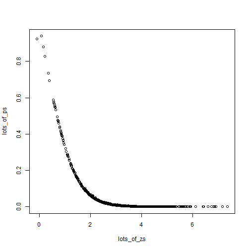

We see clearly how z-scores (x-axis) map to p-values (y-axis). This is what Gelman means by a non-informative, highly non-linear transformation of the data. While the difference in z-scores (1 to 2) for example, does not seem that great, the associated difference in p-values is huge.

If we shift the null just a little and allow a small difference of 0.2, then we get the following.

plot(lots_of_zs_pos_null, lots_of_ps_pos_null)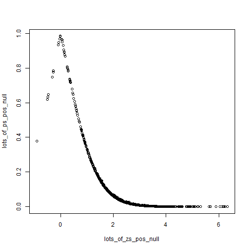

Looks similar, we still see the strong non-linearity. But to get at the second point, we can just compare the following two plots.

plot(lots_of_zs, lots_of_zs_pos_null)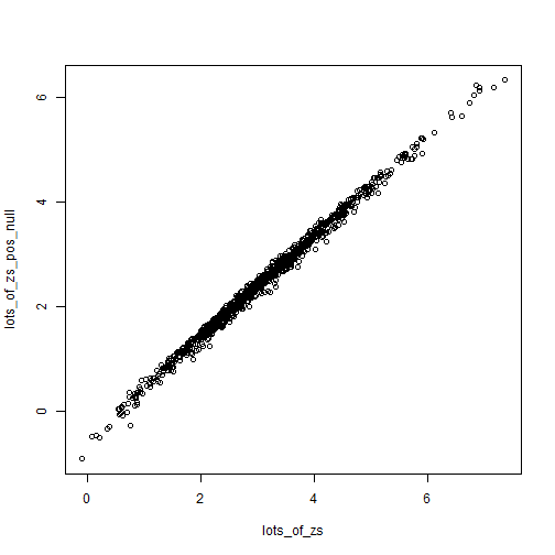

plot(lots_of_ps, lots_of_ps_pos_null)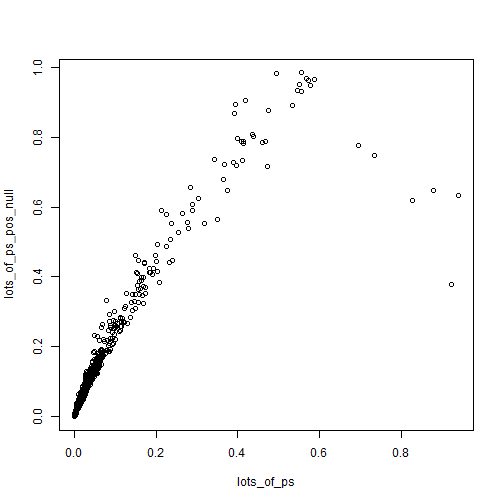

Z-scores are somewhat robust to small changes in the null (from 0 to 0.2), while p-values can swing wildly. Of course what we end up caring about is the values close to 0.05 for some reason.

sig_zero_null <- which(lots_of_ps < 0.1)
plot(lots_of_zs[sig_zero_null],
     lots_of_zs_pos_null[sig_zero_null])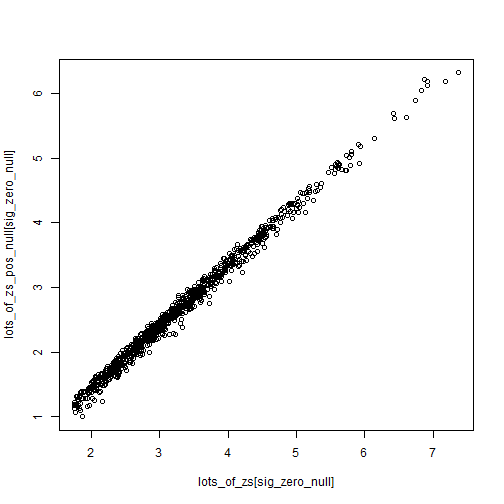

plot(lots_of_ps[sig_zero_null],
     lots_of_ps_pos_null[sig_zero_null])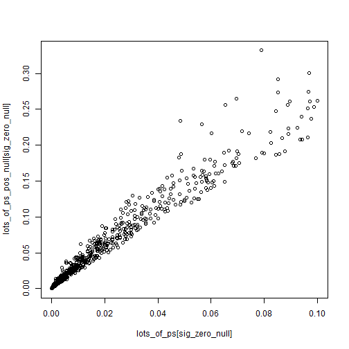

P-values magnify the reliance upon a very specific null of 0.